Fourier Analysis

Quadratures

Quadratures

Introduction

A quadrature is just a name we use to describe methods of numerical integration

In this chapter we will look at some simple methods such as the trapezium rule, which you will already be familiar with and then we will consider some more sophisticated developments, such as Simpson's and Boole's rule, which interpolate function points with polynomials of increasing degree

Finally we will look at Gaussian quadratures where the assumption of evenly spaced abscissa points is dropped and a more general form of quadrature is developed which can produce remarkably accurate results with relatively little calculation

Very basic quadrature methods

The most basic form of numerical integration is called the left point rule: In this case we simply divide the function into intervals of width $\Delta x$ and then add up the area of the rectangles width: $\Delta x$ and height: $f(x_i)$, where $x_i$ is the value of $x$ at the left of the interval

This gives: $\int_{a}^{b}f(x) dx \approx \Delta x \times \left(f(x_0)+f(x_1)+...+f(x_{n-1})\right)$

where $a=x_0$, $b=x_n$ and the $x_i$s are evenly spaced across the interval.

The right point rule and the mid-point rule follow by analogy

Clearly these methods are very primitive and it is easy to improve on them

The Trapezium Rule

The trapezium rule represents the first level of sophistication in the numerical calculation of integrals

consider the problem of how to calculate the area under the curve: $y=e^{-x} \times sin x$ between $0$ and $\pi$

The following graph shows how we could use a series of trapeziums to estimate this integral

We can easily see that the area under the trapeziums reduces to:

$A=\frac{\pi}{8} \times \left(f(0) + 2f(\frac{\pi}{4}) + 2f(\frac{\pi}{2}) + 2f(\frac{3\pi}{4}) + f(\pi) \right)$

So more generally the trapezium rule is given by:

$\int_{a}^{b} f(x) dx \approx \frac{\Delta x}{2} \times \left(f(x_0)+2f(x_1)+2f(x_2)+...+2f(x_{n-1})+f(x_{n})\right)$

Write a VBA routine to approximate the integral of a general function between abscissas $a$ and $b$ with any given number of intervals using the trapezium rule

Approximate the area under $y=e^{-x} \times sin x$ between $0$ and $\pi$ using 4, 12 and 120 intervals

Simpson's Rule

Suppose instead of fitting straight line segments to our function we attempt to find a better fit by fitting quadratic segments

Look at the same function below (grey) with two black quadratics fitted to the first three and last three calculated function points

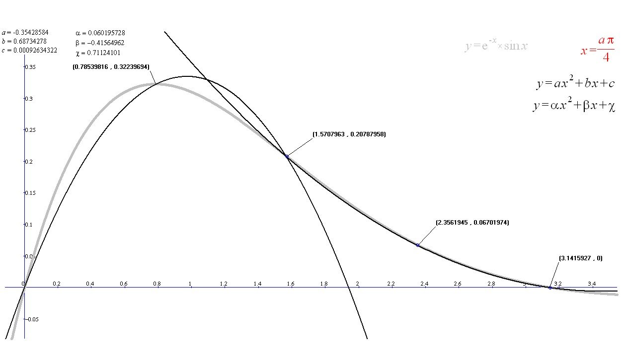
By considering a function $f$ on the interval $[-\theta, \theta ]$ and using abscissa points $-\theta$, $0$ and $\theta$, calculate the quadratic which will interpolate the three points

Using basic calculus, calculate the area under this quadratic on the interval $[-\theta, \theta ]$ as a function of $\theta$, $f(-\theta)$, $f(0)$ and $f(\theta)$

This leads us to Simpson's Rule which is stated generally as:

$\int_{a}^{b} f(x) dx \approx \frac{\Delta x}{3} \times \left(f(x_0)+4f(x_1)+2f(x_2)+4f(x_3)+...+2f(x_{n-2})+4f(x_{n-1})+f(x_{n})\right)$

Write a VBA routine to approximate the integral of a general function between abscissas $a$ and $b$ with any given number of intervals using Simpson's Rule

Approximate the area under $y=e^{-x} \times sin x$ between $0$ and $\pi$ using 4, 12 and 120 intervals using Simpson's Rule (2,6 and 60 quadratic segments)

Simpson's three eighths Rule

The next level is to fit cubic segments

Look at the same function again (grey) with the red cubic fitted to four calculated function points

The principles are exactly the same but the algebra is a bit more complicated, so Simpson's 3/8ths Rule over a $3\Delta x$ interval can be expressed as:

$\int_{a}^{b} f(x) dx \approx \frac{3\Delta x}{8} \times \left(f(x_0)+3f(x_1)+3f(x_2)+f(x_3)\right)$

Write a single VBA routine to approximate the integral of a general function between abscissas $a$ and $b$ with any given number of intervals and allowing the user to choose between the methods given so far

Approximate the area under $y=e^{-x} \times sin x$ between $0$ and $\pi$ using 3, 6, 12 and 120 intervals using Simpson's 3/8ths Rule

Boole's Rule

The next level is to fit quartic segments

This time the interpolating function is a quartic

The principles are again the same, so Boole's Rule over $4\Delta x$ interval can be expressed as:

$\int_{a}^{b} f(x) dx \approx \frac{\Delta x}{45} \times \left(14f(x_0)+64f(x_1)+24f(x_2)+64f(x_3)+14f(x_4)\right)$

Extend your VBA routine to include Boole's Rule

Approximate the area under $y=e^{-x} \times sin x$ between $0$ and $\pi$ using 4, 12 and 120 intervals using Boole's Rule

Programming Extensions

There are a number of things you should now do to tidy up your routine

Gaussian Quadratures

Gaussian Quadratures

So far all of our methods have assumed that the abscissa points have been equally spaced along the $x$-axis

We could have changed this if we wanted but there seemed little point and it would have made the algebra more complicated

The question therefore arises: Can we improve the speed or accuracy of our routine by using a different set of abscissa points?

The answer is YES and the set of methods we can use are referred to as Gaussian quadrature

General Considerations

In general all quadrature methods are based on the formula:

$\displaystyle\int_{a}^{b}f(x)dx\approx \displaystyle\sum_{i=1}^{n}\omega_i f(x_i)$

Where $\omega_i$ are a set of weights and $x_i$ are a set of abscissa points

As we are now free to choose $2n$ values we should be able to approximate our integral much more accurately - in fact if we motivate our selection of $\omega_i$ and $x_i$ by fitting polynomials then this method will calculate the integral of an order $2n-1$ polynomial exactly

2 Point Gaussian Quadratures

W.l.o.g we work on the interval $[-1, 1]$

We wish to find $\omega_1$, $\omega_2$, $x_1$ and $x_2$ such that

$\displaystyle\int_{-1}^{1}f(x)dx \equiv \displaystyle\sum_{i=1}^{2}\omega_i f(x_i)$, for a cubic $f(x)$, i.e.:

$\displaystyle\int_{-1}^{1} a_0+a_1x+a_2x^2+a_3x^3dx \equiv \omega_1 f(x_1) + \omega_2 f(x_2)$, i.e. this relation must hold for all choices of $a_i$

We proceed with basic calculus

$\left[ a_0x+\frac{a_1x^2}{2}+\frac{a_2x^3}{3}+\frac{x_3x^4}{4} \right]_{-1}^{1} \equiv \omega_1 f(x_1) + \omega_2 f(x_2)$

$a_0(1-(-1)) + a_1\frac{1^2-(-1)^2}{2} + a_2\frac{1^3-(-1)^3}{3} + a_3\frac{1^4-(-1)^4}{4} \equiv \omega_1 f(x_1) + \omega_2 f(x_2)$

$2a_0 + \frac{2}{3}a_2 \equiv \omega_1 \left(a_0+a_1x_1+a_2x_1^2+a_3x_1^3\right)+ \omega_2\left(a_0+a_1x_2+a_2x_2^2+a_3x_2^3\right)$

$2a_0 + \frac{2}{3}a_2 \equiv a_0(\omega_1 + \omega_2) + a_1(\omega_1 x_1 + \omega_2 x_2) + a_2(\omega_1 x_1^2 + \omega_2 x_2^2) + a_3(\omega_1 x_1^3 + \omega_2 x_2^3)$

As this is an identity we can match the co-efficients of the $a_i$

$a_0$: $2 = \omega_1 + \omega_2$

$a_1$: $0 = \omega_1 x_1 + \omega_2 x_2$

$a_2$: $\frac{2}{3} = \omega_1 x_1^2 + \omega_2 x_2^2$

$a_3$: $0 = \omega_1 x_1^3 + \omega_2 x_2^3$

The best way to solve these equations is guess and check as follows:

as symmetry seems likely assume $\omega_1 = \omega_2$ therefore $\omega_1 = \omega_2 = 1$

$a_1$ gives $x_1 = -x_2$

$a_2$ gives $\frac{2}{3} = \omega_1 x_1^2 + \omega_2 x_2^2 = 2 x_1^2$

so $3x_1^2-1=0$ - this is the Legendre Polynomial order 2

w.l.o.g. $x_1=-\sqrt{\frac{1}{3}}$ and $x_2=\sqrt{\frac{1}{3}}$

Calculate $\displaystyle\int_{-1}^{1} 2+6x-3x^2+x^3dx$, both analytically and using 2 point Gaussian quadrature

The last thing we need to do to make our method useful is to drop the requirement to work on the $[-1, 1]$ interval

There are two additional things we need to consider to to this:

Calculate $\displaystyle\int_{5}^{10} 2+6x-3x^2+x^3dx$, both analytically and using 2 point Gaussian quadrature

n Point Gaussian Quadratures

We could repeat the above exercise for 3 and then 4,5 ,6 etc points. The algebra does get complicated, but fortunately we have the following theorem:

If we perform n point quadrature by selecting the $x_i$ to be the roots of the Legendre Polynomials and the weighting function to be $\omega_i = \frac{2}{(1-x_i^2)(P'_n(x_i))^2}$, where $P'_n(x_i)$ is the differential of the $n^{th}$ Legendre Polynomial then our resulting quadrature will integrate polynomials of order $2n-1$ exactly

We do not attempt to prove this result here - but the above analysis is the proof of this result for 2 point quadrature. You can see how the Legendre Polynomial arises in the above analysis

The Legendre Polynomials are defined by: $P_n(x)=\frac{1}{2^n} \displaystyle\sum_{k=0}^{n} \left({n \choose k}^2 \times (x-1)^{n-k} \times (x+1)^k\right)$

Formula 98 files are Legendre Polynomials and Legendre Polynomials wi

Calculating $P'_n(x)$ is a simple application of the product rule

So we can see that the first few of the Legendre Polynomials are:

Produce a spreadsheet which draws graphs of each of the Legendre Polynomials

What do you notice about the dispersion of the roots?

Now compare the roots of the n-th order Legendre Polynomial with the value of $x=cos \left( \frac{(i-0.25) \pi}{n+0.5} \right)$

How might we use the formula: $x=cos \left( \frac{(i-0.25) \pi}{n+0.5} \right)$

To produce initial estimates of the roots so we can then use Newton Rhapson to produce our exact roots

1. Develop a VBA function which can perform an n point Gaussian quadrature over a given interval for any given function

2. change your code so that the calculation of the Legendre Polynomial roots is only calculated once, however many times the routine is called

Hint: you will need to store the $\omega_i$ and $x_i$ values outside of the function so that they have module wide scope and use a boolean array to determine whether the values have already been calculated or not

3. Use 2, 4, 6, 8 and 10 point Gaussian quadrature to calculate $\displaystyle\int_{0}^{\pi} sin x dx$

The answer spreadsheet : quadrature.xls is here

Fourier Analysis

Fourier Analysis

Fourier analysis allows us to convert waveforms into spectral densities and back again

In excel draw a graph of $y=sin x$

On the same axes draw $y=sinx + \frac{sin 2x}{2}$

Create a VBA function for $y=\displaystyle\sum_{k=1}^{n} \frac{sin kx}{k}$ and again plot on the same axes for different values of $n$

You can soon see that as $n \rightarrow \infty$ this function becomes a sawtooth wave

This raises the question: If we started with the sawtooth wave wave could we calculate the co-efficients

This is where fourier analysis comes in

For our purposes we will skip Fourier series and go onto the continuous Fourier transform

The fourier tranform $\hat{f}$ of an integrable function $f:\Re \rightarrow C$ is given by

$\hat{f}(\xi)=\displaystyle\int_{-\infty}^{\infty}f(x) e^{2 \pi ix \xi} dx$

$f$ is the original wave function of time $x$ and $\hat{f}$ is the spectral density of frequency $\xi$

The process can be inverted by the inverse transform:

$f(x)=\displaystyle\int_{-\infty}^{\infty} \hat{f}(\xi) e^{-2 \pi ix \xi} d\xi$

The above formulas look rather daunting but we start by breaking them down with Euler's formula:

$e^{ix}=cos x + i sin x$

Write a VBA function which takes a function $f$, a parameter $\xi$, specifies bounds $a$ and $b$ outside of which the function will be close to zero, and returns the Fourier transform $\hat{f}(\xi)$

Fast Fourier Transform
Discrete Fourier transform

Discrete Fourier transform

Before we look at the algorithm for the Fast Fourier transform we must understand the discrete Fourier transform.

This is simply the discretised version of the Fourier transform - the numerical integration version.

Instead of performing the integral: $\hat{f}(\xi)=\displaystyle\int_{-\infty}^{\infty}f(x) e^{2 \pi ix \xi} dx$ we perform the sum $\hat{f}(\xi)=\displaystyle\sum_{x=1}^{n}f(x) e^{2 \pi i \frac{x}{n} \xi}$

The following diagrams illustrate how this works to produce the spectral density of the function

You should note that there are alternative ways of setting this up:

  • We could go from x=1/n to 1 and leave the divide by n out
  • We could have the $e^{-}$ in the Fourier transform and the positive in the inverse transform

The principles are the same in each case

The spreadsheet DFT.xls shows how a discrete Fourier transform can be performed in excel

Fast Fourier Transform

Fast Fourier Transform

The Fast Fourier Transform takes advantage of the fact that the discrete Fourier transform set up as above allows us to repeat the use of the $e^{2 \pi i x \xi}$ and so avoid having to keep calculating a computationally expensive number

We then divide each transform into an odd and an even section and show how different transforms can be calculated from already calculated numbers.

The following slides illustrate the point

Fast Fourier transform Exercise
HARD (I will try and demonstrate before end of term)

Generate 1024 numbers in excel with some sort of periodicity

  • Write a visual basic subroutine (behind a button) which takes these values into an array
  • Calculate all the $e^{2\pi i \frac{x}{n}}$ values you will need, just using separate $x$ and $y$ values
  • Use the fastest algorithm you can to calculate the Fourier transform $\hat{f}(\xi)$ for all values of $\xi \in [1..1024]$
  • Output back to excel the Fourier transform you have created (the modulus of the complex numbers)
  • Test your routine with different signal numbers $f(x)$

The issue here lies in how to structure the arrays to carry the required information in the FFT algorithm